In this part, we create the “business logic” of our basic app. We would like to retroactively analyze our past spendings and to select transactions, which we need to cut in order to achieve a certain savings level. Under the hood, we will have a small optimization problem, which we solve with an open-source solver. Note, that this problem can be solved in multiple ways, and probably one can write a simple deterministic algorithm to find the optimal solution. However, our usage of MIP solver makes the approach extendable: we can easily add additional rules for optimization without making major changes to the algorithm. Let’s take a look!

Relative importance of transactions

For optimization to make sense, we as users may want to specify the relative importance of transactions. In the end, we want to deduce a retroactive savings plan, and to do so we need to “cancel” some transactions. It is clear that one may save on grocery shopping, but saving on rent payments does not sound like a good idea.

Where the importance factors are coming from?

That can be user input. For each transaction type we can specify importance factor as integer value. Below are mine:

importance_factors = {"grocery":1, "fashion":2, "shopping":3, "travel":10, "rent": 1000, "unknown":10, "income":0}

Problem

You would like to understand which type of expenses you need to cut in the future in order to achieve certain savings per year. Given a savings amount X, you need to return a list of transactions with minimal total importance, which you could have cut during the current year, in order to save this amount.

Sanity rules:

• You know that there is a certain amount you need to spend on groceries (you need to eat)
• Every season you need to spend a certain amount on clothing
• In general, you cannot avoid paying for household

So what we would like to have is a retroactive saving plan for our banc account: where I could have avoided additional expenses to achieve certain savings for the last year

Model

Decision

Take or not to take the corresponding transaction. Let transaction be indexed by \(n \in \mathcal{N}\). Then the decision variable, corresponding to taking or not taking transaction \(n\) is \(z_n \in \{0,1\}\)

Optimization goal, i.e. objective function

We want to minimize the total importance of all the transaction we decide to keep, to achieve certain savings goal. If \(I_n\) is the importance of transaction $n$, then our goal is to \(\begin{align*} \max \sum_{n \in N} I_n z_n \end{align*}\)

Constraints

Grocery

Well, we can never actually cut on grocery entirely. This retroactive savings plan would look ridiculous if some of the weeks will have 0 EUR spent on the grocery. That’s why we introduce a minimum bound for grocery expenses per week

where \(\mathcal{N}^G_{w}\) is a set of transactions of type grocery, happening in a specific week \(w\), \(B^G\) is the minimum weekly allowance for grocery, which we find feasible (user input).

Now, there is a little trick here. If we keep constraint as it is, it may happen to be infeasible for some weeks. Imagine, one week you were paying all grocery expenses by cash, and thus they do not appear in your transactions. Yet, you ask the solver to find a solution, which exceeds your minimum allowance for groceries that week. That’s simply impossible! That’s why we modify our formulation, to account for such cases:

and here \(\sum_{n \in \mathcal{N}^G_{w}}\) accounts for maximum transaction cost in grocery in week \(w\) which you see in data. If this is above the allowance limit, the latter will be used in the constraint. If it is smaller, we will use the observed cost from data as a lower bound limit.

Household

We simply cannot avoid paying the rent. We would like our model to disallow saving plans which remove rent payments: \(\begin{align*} z_n = 1, \quad \forall n \in \mathcal{N}^H, \end{align*}\) where \(\mathcal{N}^H\) is the set of transactions corresponding to rent payments.

Savings

What we would like to know in the end is where do we need to cut, to have a certain savings number. We can put it is a target, or as a constraint. I’ve chosen the latter: \(\begin{align*} \sum_{n \in N} C_n (1-z_n) >= S, \end{align*}\)

and here \(S\) is our overall savings target. If the target is given as a percentage of the total expenses \(P\), then \(S = P * \sum_{n \in N} C_n\)

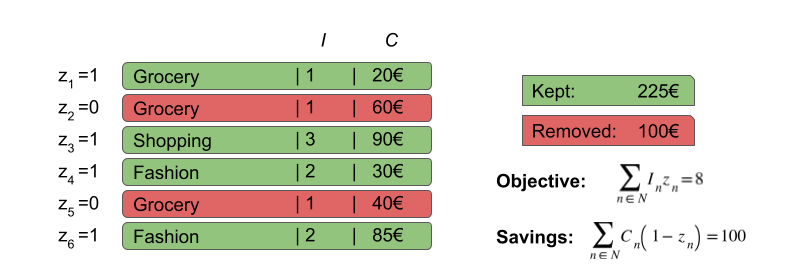
Solution example

In the picture below, we see a small dataset, on which the problem is already solved. We can see that 2 transactions were removed, amounting to the total saving of 100 EUR. The objective value (total importance of kept transaction) equals 8.

Model creation with PuLP

PuLP is an LP modeler written in Python. It comes with open-source CBC solver, which makes it an easy choice to start with. We create a basic model object, already specifying optimization sense (maximization).

model = pulp.LpProblem("Profit_maximizing_problem", constants.LpMaximize)

Decision variables

The model has two essential parts: variables and constraints (which describe a relation between variables). Typically, the usual first step with the implementation of the optimization model is to define variables. In our case, this is a set of binary variables (having values 0 or 1), which describe for each transaction whether it should be kept or removed from the retroactive savings plan, \(z_n \in \{0,1\}\)

decision_vars = pulp.LpVariable.dicts(
    "Transaction", selected_year.index, 0, 1, LpInteger)

Objective

We can already define the objective function, i.e. the function which we ask our solver to maximize. In our problem, this is the total importance of transactions we decided to keep in the plan. So we simply multiply each decision variable \(z_n\) by the importance factor of the corresponding transaction, then sum them up.

objective = pulp.lpSum(
    [decision_vars[t] * selected_year.loc[t, "importance"] for t in selected_year.index]
)
model += objective

Constraints

Let’s start with the easiest constraint to formulate. We would like to always keep rent payments in our plan. This means that we want all decision variables, corresponding to rent payment transactions to be equal to 1 (i.e. we keep them)

for t in selected_year.index:
    if selected_year.loc[t, "type"] == "rent":
        model += decision_vars[t] == 1

Now we have a savings constraint to add. What we want is to make sure that certain savings are achieved. We opted for relative savings input. Note, we need to take the absolute value of “Debit”, because the original data contains negative values there. We could have dealt with it in the data preparation step, but this will work as well

total_expenditure = abs(selected_year.sum()["Debit"])
savings_constraint = (
    pulp.lpSum([decision_vars[t] * abs(selected_year.loc[t, "Debit"]) for t in selected_year.index])
    <= (1 - savings) * total_expenditure
)
model += savings_constraint

Now comes the tricky one: grocery expenses constraint. We would like to make sure that our savings plan does not deliver ridiculous outcomes and cuts food expenses to 0. Thus we would like to have a lower bound on grocery expenses. In addition, we would like to make sure that this lower bound is achievable because otherwise, the model might become infeasible. E.g., if the user specifies a lower bound of 100 EUR per week, but a certain week contains transactions amounting only to 50 EUR, the lower bound for such week should be minimum between bound and transactions sum, which is 50 EUR in the described case.

We start with computing current grocery expenses per week:

agg_per_week = selected_year[selected_year["type"] == "grocery"].groupby("week").sum()

Next, we add weekly constraints:

for w in range(52):
        if w in agg_per_week.index:
            week_grocery_spending = abs(agg_per_week.loc[w, "Debit"])
            model += pulp.lpSum(
                [
                    decision_vars[t] * abs(selected_year.loc[t, "Debit"])
                    if (selected_year.loc[t, "week"] == w) and (selected_year.loc[t, "type"] == "grocery")
                    else 0.0
                    for t in selected_year.index
                ]
            ) >= min(week_grocery_spending, grocery_per_week)

Solving the model

Now we are good to solve the model. An important thing is to check model status afterward: if the solution is not optimal, most likely we would not like to use it

status = model.solve()

if LpStatus[status] == 'Optimal':
    print("Model soved optimally")
else:
    print(f"Model solving was unsuccessful with status {LpStatus[status]}")

Parsing model output: simply for each transaction assign the value of the decision variable. In addition, we check the value of the objective

solution = pd.Series(
    [
        decision_vars[t].varValue if decision_vars[t].varValue is not None else 1
        for t in selected_year.index
    ],
    index=selected_year.index,
    name="solution",
    dtype=np.int64,
)
objective = pulp.value(model.objective)

And finally merging it with our inputs dataframe. Now for each transaction, we have a solution value, which tells us whether this transaction should be kept (1) or removed (0) in our retroactive savings plan.

solved_data = selected_year.join(solution)

Code

This code can be found in repository

The whole series of posts

1. Budget optimization intro
2. Data preparation
3. Data visualizaion
4. Optimization model
5. Make it work